“Essentially, all models are wrong, but some are useful.” George E. P. Box
Introduction
This is by no means a new topic nor a particularly complex one, but I generally like to know where stuff in math or science really comes from. If you’re reading this, you are probably familiar with Linear Regression or Least Squares Regression (or whatever other name you’ve heard it called). The premise is that for each data point in our population, we measure some label \(y_i\) (for simplicity we take this to be scalar) and the values of some set of features associated to this label \(\mathbf{x}_i \in \mathbb{R}^n\). We can then aim to fit some function \(f: \mathbb{R}^n \rightarrow \mathbb{R}\) such that \(f(\mathbf{x}_i) = \hat{y}_i \approx y_i\). In Linear Regression, we limit the space of such models \(f\) to that of models which are linear (or affine) in the summation coefficients \(\mathbf{\theta}\):
\[ \begin{align} \hat{y}_i = \theta_1 x^{(i)}_1 + \theta_2 x^{(i)}_2 + ... = \mathbf{\theta} \cdot \mathbf{x}_i \end{align} \]
We typically also include a constant bias or offset term \(\theta_0\) which, to keep the dot product structure, we encode by appending a \(1\) to the end of our feature vector \(\mathbf{x}_i\). We can actually also capture non-linearities in the features - although \(f\) must always be linear in the parameters \(\mathbf{\theta}\) - by appending powers or other non-linear functions of the features to \(\mathbf{x}_i\).
We can think of this dot product as projection of \(\mathbf{x}_i\) onto some direction \(\mathbf{\theta}\) and thus performing a dimensionality reduction down to 1D (ie: a line). The value of \(\hat{y}_i\) is then the 1 variable required to index a datum \((y_i, \mathbf{x}_i)\) along this line.
As good statisticians, we might measure \(m\) such outputs \(y_i\) and for each, their corresponding feature vector \(\mathbf{x}_i\). It is convenient to concatenate our \(y_i\) into a column vector \(\mathbf{y} \in \mathbb{R}^m\) and our \(\mathbf{x}_i\) vectors as rows of a matrix \(X \in \mathbb{R}^{m \times n}\). We assume that there exists some optimal \(\mathbf{\theta}^{\ast}\) such that the true labels \(\mathbf{y}\) can be expressed as:
\[ \begin{align} \mathbf{y} = \matrix{X} \mathbf{\theta}^{\ast} \end{align} \]
This lends a useful geometric interpretation, although that isn’t the focus of this post. We can consider the vector of labels as being expressed as a linear combination of the column space of \(\matrix{X}\). Each vector in this column space can be interpreted as the vector of one feature’s values for all samples in our dataset. This linear algebra interpretation quickly points to where problems might arise - maybe \(\mathbf{y}\) lies outside the span of the column-space. Another common problem is having high colinearity between vectors in this column space which renders the linear mapping represented by the matrix \(\matrix{X}\) non-invertible - this can harm numerical stability of solutions or simply make the solution non-existent in the extremal case. We will address this issue later.
I personally prefer working in index notation (the arguments scale easily to arbitrary dimensions) so I’ll stick to that. Now that we have our equations formalised, we turn to a probabilistic interpretation to motivate the least squares optimisation.
Why Least Squares?
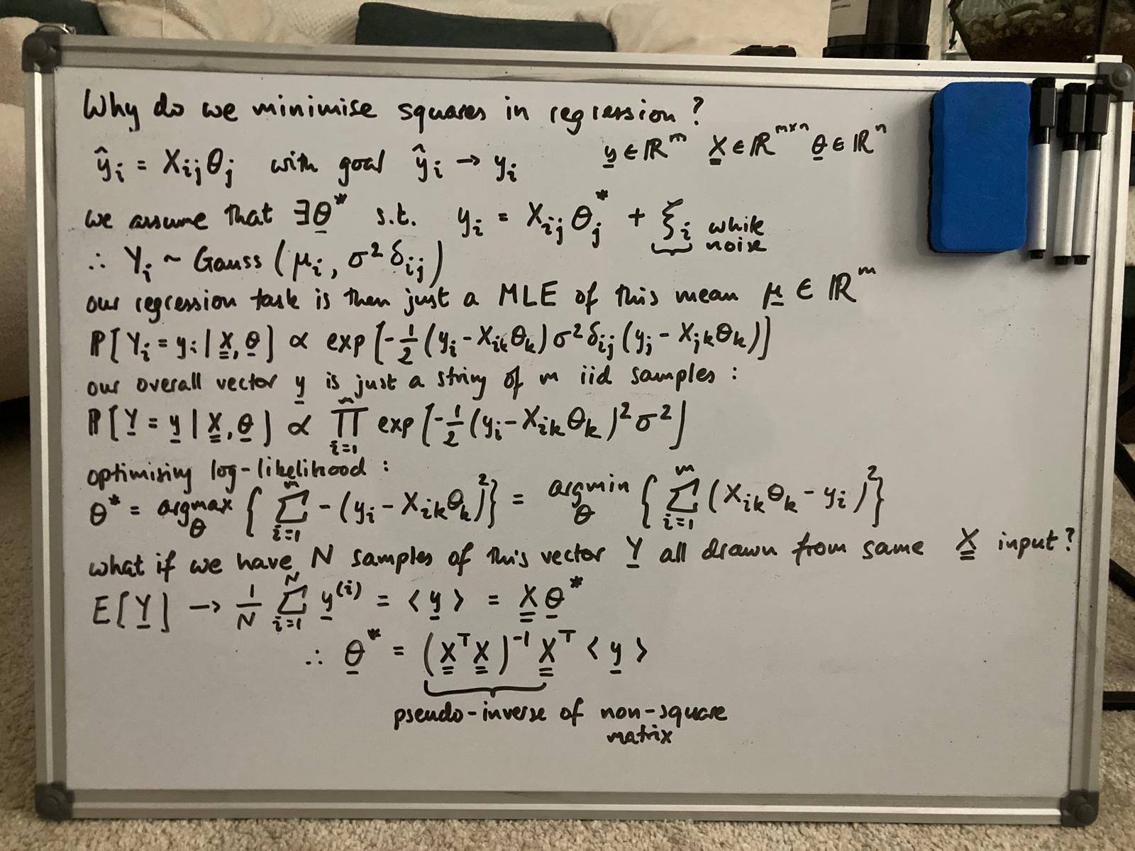
We define our dataset to be \(\mathcal{D} = \{(y_i, \mathbf{x}_i)\}_{i=1}^{N}\). In regression, we generally take the labels \(y_i\) to be random variables whilst the feature vectors \(\mathbf{x}_i\) are treated as exact non-random quantities (this is of course a modelling over-simplification). We must assume some randomness in \(y_i\) otherwise the conditional distribution over the labels collapses to a delta cone which we cannot make much use of. It should also be intuitively sensible to assume that our label measurements will be noisy. For the Ordinary Least Squares (or OLS) solution, we simply seek to maximise the likelihood of our probabilistic labels given our choice of parameters.
We generally take the noise in our labels to be zero mean-gaussian. This is equivalent to writing \(y_i = \mu_i + \xi_i\) where \(\xi_i \sim \mathcal{N}(0, \sigma^2)\) and \(\mu_i = X_{ij}\theta_j\). This is sumarrised below.
\[ \begin{align} Y_i \sim \mathcal{N}(X_{ij}\theta_j, \sigma^2 \delta_{ij}) \end{align} \]
For each datum \(y_i\) there is a corresponding distribution. All have the same variance (by our assumption of the noise) but the mean will be different - importantly, the mean is always coupled to the input feature vector. Equivalently, we can think of the concatenated vector of measured outputs \(\mathbf{y}\) as being a sample from:
\[ \begin{align} \mathbf{Y} \sim \mathcal{N}(\matrix{X}\mathbf{\theta}, \sigma^2 \mathbb{I}) \end{align} \]
Our goal parameter \(\theta_j^{\ast}\) is inside the distribution’s mean. If we had many such vectors \(\mathbf{y}_i\) all drawn from the same data matrix \(\matrix{X}\), the job of finding the mean would be straightforward (we’ll get back to this later). We generally only measure one such \(\mathbf{y}\). Writing out this gaussian distribution over our labels \(y_i\) we have:
\[ \begin{align} p_{\matrix{X}, \mathbf{\theta}}(y_i) \propto \exp\Bigg[-\frac{1}{2} &(y_i - X_{ik}\theta_k) (\sigma^2 \delta_{ij})^{-1} (y_j - X_{jk}\theta_k) \Bigg] \end{align} \]
Note that I am choosing to write \(p_{\matrix{X}, \mathbf{\theta}}(y_i)\) rather than \(p(y_i | \matrix{X}, \mathbf{\theta})\). This is simply to make clear what is and isn’t random in the model (most texts will opt for the latter notation).
Now that we have probabilities, we can turn to the principle of maximum likelihood. In our case, this constitutes finding the parameter \(\mathbf{\theta}\) for our distribution such that the observed data \(\mathbf{y}\) is maximally likely (under our choice of distribution). This optimal parameter is known as the maximum likelihood estimator (MLE) \(\mathbf{\theta}_{MLE}\). If our \(m\) samples are iid, this likelihood over the whole dataset is simply the product of each label’s likelihood \(p_{\matrix{X}, \mathbf{\theta}}(\mathbf{y}) = \prod_{i=1}^m p_{\matrix{X}, \mathbf{\theta}}(y_i)\). By the monotonicity of the logarithm, we can equivalently maximise the logarithm of this product (a standard trick). Omitting constant factors like the variance \(\sigma^2\) or the normalisation factors, we have:
\[ \begin{align} \mathbf{\theta}_{MLE} &= \arg\max_{\theta} \prod_{i=1}^m p_{\matrix{X}, \mathbf{\theta}}(y_i)\\ &= \arg\max_{\theta} \sum_{i=1}^m \log p_{\matrix{X}, \mathbf{\theta}}(y_i) \\ &= \arg\max_{\theta} \left\{ \sum_{i=1}^{m} -\frac{1}{2} (y_i - X_{ik} \theta_k)^2 \right\} \\ &= \arg\min_{\theta} \left\{ \sum_{i=1}^{m} (y_i - X_{ik} \theta_k)^2 \right\} \end{align} \]
This is now the familiar form of the problem with solution \(\mathbf{\theta} = (\matrix{X}^{\top} \matrix{X})^{-1}\matrix{X}^{\top} \mathbf{y}\). Now we can revisit the suggestion of arriving at this answer by collecting lots of sample vectors \(\mathbf{y}_i\) (all from the same data matrix \(\matrix{X}\)) and finding their arithemtic mean. The process would like like this:
\[ \begin{align} \langle \mathbf{y} \rangle &= \frac{1}{N} \sum_{i=1}^{N} \mathbf{y}_i \\ &= \matrix{X}\mathbf{\theta}_{MLE} \\ \rightarrow \mathbf{\theta}_{MLE} &= (\matrix{X}^{\top} \matrix{X})^{-1}\matrix{X}^{\top} \langle \mathbf{y} \rangle \end{align} \]
Seeing as our vectors \(\mathbf{y}_i\) are sampled from a gaussian, the arithmetic mean turns out to be the MLE for the gaussian mean. Unfortunately, this process is quite inconvenient as the pre-requisite that the data matrix \(\matrix{X}\) be identical over the repeated samples of \(\mathbf{y}_i\) can be difficult to enforce in real world data collection. It also increases the memory requirements of any algorithm performing this regression which is generally undesirable.
Incorporating Priors
We will now promote the parameters \(\theta_j\) to random variables. Suppose we are trying to predict height in a sample of people. We might collect feature data for each person including: parent height, person weight, parent weight, …, annual salary etc. Intuitively, some feature variables will be more important and require larger summation coefficient or weighting than others. More generally, we want to make use of any prior knowledge of the distribution of \(\mathbf{\theta}\). This is known as regularisation. We now require a more rigorous Bayesian treatment of the problem. Ultimately, we want to extract a posterior distribution over our parameters \(\mathbf{\theta}\) given the observed dataset \(\mathcal{D}\).
We first require the standard Bayesian inference step to reach the posterior:
\[ \begin{align} p(\mathbf{\theta} | \mathcal{D}) &= \frac{p(\mathcal{D} | \mathbf{\theta}) p(\mathbf{\theta})}{p(\mathcal{D})} \\ &\propto p(\mathbf{\theta})\prod_{i=1}^m p_{\matrix{X}}(y_i | \mathbf{\theta}) \end{align} \]
When optimising in the Bayesian framework, we can often drop the \(p(\mathcal{D})\) term as it is not a function of \(\mathbf{\theta}\) and thus will vanish under any differentiation. Our estimator will now be the maximum a-posteriori estimator (MAP) rather than the MLE. We could alternatively evaluate the exact posterior distribution \(p(\mathbf{\theta} | \mathcal{D})\) and evaluate the expectation \(\mathbb{E}[\mathbf{\theta} | \mathcal{D}]\). There are few other exact distributions we can extract using the Bayes rule - such as \(p_{\mathbf{x}^{\ast}}(y^{\ast} | \mathcal{D}) = \int p_{\mathbf{x}^{\ast}}(y^{\ast} | \mathcal{D}, \mathbf{\theta})p(\mathbf{\theta} | \mathcal{D}) d\mathbf{\theta}\), the posterior predictive distribution. Unfortunately these distributions are often computationally expensive to recover due to the integrals involved. We thus proceed with the simpler MAP point estimator.
\[ \begin{align} \mathbf{\theta}_{MAP} &= \arg\max_{\theta} p(\mathbf{\theta} | \mathcal{D}) \\ &= \arg\max_{\theta} \{ p_{\matrix{X}}(\mathbf{y} | \mathbf{\theta}) p(\mathbf{\theta}) \} \end{align} \]
A common assumption is that the weights are also iid gaussian with \(\theta_j \sim \mathcal{N}(0, \tau^2)\) thus for all \(n\) weights in our weight vector we have that \(p(\mathbf{\theta}) \propto \prod_{j=1}^{n} \exp\Bigg[\frac{\theta_j^2}{2\tau^2} \Bigg]\). Evaluating the posterior gives us:
\[ \begin{align} p(\mathbf{\theta} | \mathcal{D}) &\propto \prod_{i=1}^{m} \exp\Bigg[-\frac{1}{2\sigma^2} (y_i - X_{ik}\theta_k)^2 \Bigg] \prod_{j=1}^{n} \exp\Bigg[-\frac{\theta_j^2}{2\tau^2} \Bigg] \\ \mathbf{\theta}_{MAP} &= \arg\max_{\theta} \left\{ \sum_{i=1}^{m} -\frac{1}{\sigma^2} (y_i - X_{ik} \theta_k)^2 + \sum_{j=1}^{n} -\frac{\theta_j^2}{\tau^2} \right\} \\ &= \arg\min_{\theta} \left\{ \sum_{i=1}^{m} (y_i - X_{ik} \theta_k)^2 + \lambda \sum_{j=1}^{n} \theta_j^2 \right\} \\ \text{where } \lambda &= \frac{\sigma^2}{\tau^2} \end{align} \]
This is the Ridge regression which we interpret as punishing large coefficients (in a loss function sense). The analytic solution is now \(\mathbf{\theta} = (\matrix{X}^{\top} \matrix{X} + \lambda \mathbb{I})^{-1}\matrix{X}^{\top} \mathbf{y}\). A full bias-variance analysis (a topic for another post) reveals that this estimator is (unsurprisingly) biased but with lower variance. By restricting our search for parameters which also satisfy our assumption of the underlying parameter distribution, the spread of our optimal parameter will intuitively be smaller at the cost of bias.
Another common assumption of the underlying distribution is the Laplace or double-exponential assumption. This corresponds to \(p(\theta_j) = \frac{1}{2b}\exp [-\frac{|\theta_j|}{b}]\). This symmetric distribution is much narrower than a gaussian with a much sharper gradient around zero. This shape is useful if we assume that not only are weights evenly distributed about zero, but many weights are exactly zero. Such an assumption is present in cases where we know that only a small subset of our feature space is relevant at all (but we don’t know apriori which features these are so we measure all of them anyway). An identical treatment to the above discussion on Ridge gives:
\[ \begin{align} \mathbf{\theta}_{MAP} &= \arg\min_{\theta} \left\{ \sum_{i=1}^{m}(y_i - X_{ik}\theta_k)^2 + \lambda \sum_{j=1}^{n} |\theta_j| \right\} \\ \text{where } \lambda &= \frac{2\sigma^2}{b} \end{align} \]
This is the Lasso regression which also punishes large coefficients but is less forgiving for very small ones (unlike Ridge). The absolute value function is not differentiable at zero so there is no analytic solution for \(\mathbf{\theta}\). We usually proceed by sub-gradient descent (see here).
Numerical Stability
These regularisation methods can now be seen to arise from the introduction of priors on our parameter \(\mathbf{\theta}\). The solutions they present can also be studied in a linear algebra context as improving numerical stability in cases of high colinearity between columns of the data matrix \(\matrix{X}\). We will consider the situation under Ridge regression.
I will quickly present why colinearity in the columns of a rectangular matrix can be a problem for regression. A linear mapping \(\Phi: \mathbb{R}^n \rightarrow \mathbb{R}\) is non-invertible iff \(\Phi(\mathbf{v}) = \mathbf{0}\) for some \(\mathbf{v} \neq \mathbf{0}\):
\[ \begin{align} \matrix{X}\mathbf{v} &= \mathbf{0} \\ \iff \matrix{X}^{\top}(\matrix{X}\mathbf{v}) &= \mathbf{0} \\ \iff (\matrix{X}^{\top}\matrix{X})\mathbf{v} &= \mathbf{0} \\ \end{align} \]
Thus, if \(\matrix{X}\) is rank-deficient (has colinear columns), then the square symmetric matrix \(\matrix{X}^{\top}\matrix{X}\) (which is in the regression estimator solution) is non-invertible (must have at least one zero eigenvalue). However, even in the non-extremal case of partial colinearity, we can still encounter numerical issues. We can analyse this in terms of the eigenvalues of \(\matrix{X}^{\top}\matrix{X} \equiv \matrix{S}\):
\[ \begin{align} \matrix{S} &= \matrix{U}\matrix{\Lambda}\matrix{U}^{\top} \\ \mathbf{v}^{\top}\matrix{S}\mathbf{v} &= \mathbf{v'}^{\top}\matrix{\Lambda}\mathbf{v'} \\ &= \sum_{i=1}^m \lambda_i (v'_i)^2 \\ &= \frac{1}{m}||\matrix{X}\mathbf{v}||^2 \\ \end{align} \]
In the partial colinearity case we have \(||\matrix{X}\mathbf{v}|| \ll ||\mathbf{v}||\). Thus from the equality above we see that \(\sum_{i=1}^m \lambda_i (v'_i)^2 \ll ||\mathbf{v}||^2\). We interpret this as there being directions (eigenvectors) of \(\matrix{S}\) for which the eigenvalue is very small/vanishing. This means that numerical errors in \(\matrix{S}^{-1}\) in OLS will blow up as they scale with \(\sim \frac{1}{\lambda}\).
In Ridge, our regression estimator is \((\matrix{X}^{\top} \matrix{X} + \lambda_{Ridge} \mathbb{I})^{-1}\matrix{X}^{\top} \mathbf{y}\). The addition of the \(\lambda\mathbb{I}\) term pushes any small eigenvalues away from zero. We can see this as a damping effect by writing the estimators in terms of the eigenbasis of \(\matrix{S}\) \(\{\mathbf{u}_i \}_{i=1}^n\) for \(\mathbf{u}_i \in \mathbb{R}^n\):
\[ \begin{align} \mathbf{\theta}_{OLS} &= \sum_{i=1}^n \frac{\mathbf{u}^{\top}_i \matrix{X}^{\top} \mathbf{y}}{\lambda_i} \mathbf{u}_i \\ \mathbf{\theta}_{Ridge} &= \sum_{i=1}^n \frac{\mathbf{u}^{\top}_i \matrix{X}^{\top} \mathbf{y}}{\lambda_i + \lambda_{Ridge}} \mathbf{u}_i \end{align} \]
The unstable directions are now dampened with an increased denominator in the eigenbasis expansion. We can interpret these directions rather nicely. The directions of small eigenvalues correspond to directions in \(\mathbb{R}^n\) which are nearly orthogonal to all the rows of \(\matrix{X}\). More simply, we can observe that \(\matrix{X}^{\top}\matrix{X}\) is symmetric positive semi-definite and \(\mathbb{I}\) is symmetric positive definite (SPD) thus the weighted sum of the two is SPD which guarantees the inverse exists.